Capítulo 3 Gráficos estadísticos

3.1 Histograma de frecuencias

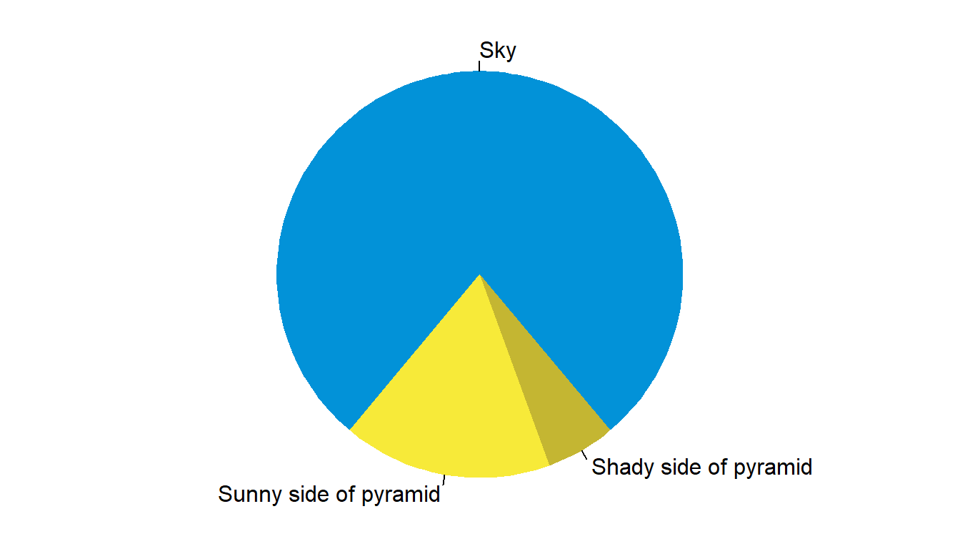
3.2 Circulares

par(mar = c(0, 1, 0, 1))
pie(
  c(280, 60, 20),
  c('Sky', 'Sunny side of pyramid', 'Shady side of pyramid'),
  col = c('#0292D8', '#F7EA39', '#C4B632'),
  init.angle = -50, border = NA
)

plot(cars)
lines(lowess(cars))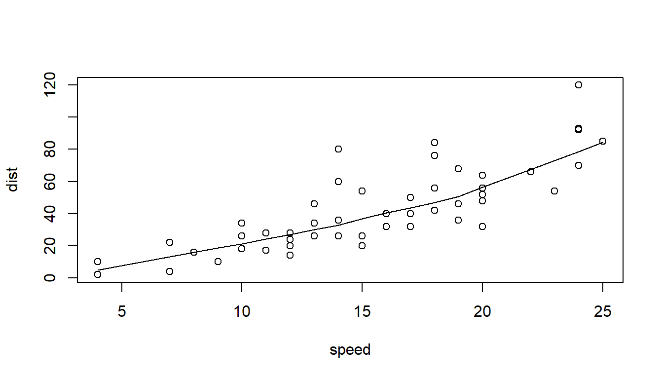

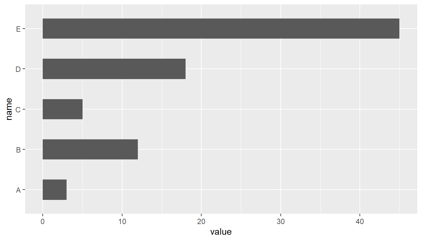
library(ggplot2)

## Warning: package 'ggplot2' was built under R version 4.1.3

# Create data
data <- data.frame(
  name=c("A","B","C","D","E") ,  
  value=c(3,12,5,18,45)
  )

# Barplot
ggplot(data, aes(x=name, y=value)) +
  geom_bar(stat = "identity", width=0.5) +
  coord_flip()